CBSE-IX-Foundation of Information Technology .
11: MS-Excel 2007
Note: Please signup/signin free to get personalized experience.
Note: Please signup/signin free to get personalized experience.
10 minutes can boost your percentage by 10%
Note: Please signup/signin free to get personalized experience.
- Qstn #9For what purpose pie charts are useful?Ans : Pie charts are useful for the following purposes:
- They convey approximate propositional relationship at a point in time.
- They compare part of a whole at a given point in time.
- Exploded portion of a pie chart emphasize a small proportion of parts.
- They convey approximate propositional relationship at a point in time.
- #Section : CLong Answer Type Questions
- Qstn #1Explain the concept of cell referencing alongwith its various types.Ans : Excel supports three types of cell referencing, which are as follows:
- Relative Every relative cell reference in formula automatically changes when the formula is copied down a column or across a row. As the example illustrated here shows, when the formula is entered (= B4 — C4) in Cell D4 then this formula copied in D5 then it will change into (= B5 — C5) related to cell.
- Absolute An absolute cell reference is fixed. Absolute references do not change if you copy a formula from one cell to another. Absolute references have dollar sign ($) like $S$9. As the shows, when the formula =C4*$D$9 is copied from row, the absolute cell reference remains as $D$9. ‘
- Mixed A mixed cell reference has either an absolute column and a relative row, or an absolute row and a relative column, e.g. $A1 is an absolute reference to column A and a relative reference to row 1. As a mixed reference is copied from one cell to another, the absolute reference stays the same but the relative reference changes.
- Relative Every relative cell reference in formula automatically changes when the formula is copied down a column or across a row. As the example illustrated here shows, when the formula is entered (= B4 — C4) in Cell D4 then this formula copied in D5 then it will change into (= B5 — C5) related to cell.
- Qstn #2Explain any five functions that can be used in a worksheet.Ans : 1. SUM Function
This function, as clear from name, is used to add all the values provided as argument and to display the result in the cell containing function.
Argument Type All Numbers Return Type Number
Syntax = SUM(numberl, number2, )
e.g. if you want to display the sum of values of cells Al, A2, A5 and A6 in cell A9, then you need to simply type = SUM(A1,A2,A5,A6) in cell A9 and press Enter.
The sum will be displayed in cell A9. If you want to add a range of values, then provide that range in SUM function as an argument.
e.g. if you want to add values from Al to A5, then write like =SUM(A1:A5).
- If an argument is an array or reference, only numbers in that array or reference are counted. Empty cells, logical values or text in the array or reference are ignored.
- If any arguments are error values or if any arguments are text that cannot be translated into numbers, Excel displays an error.
2. AVERAGE Function
This function calculates the average of all the values provided as argument to this function.
Argument Type All Numbers Return Type Number
Syntax = AVERAGE(numberl, number2, )
e.g. to calculate the average of the values of range starting from Al to A5 in cell B9, you need to write = AVERAGE(A1:A5) in cell B9. - If an argument is an array or reference, only numbers in that array or reference are counted. Empty cells, logical values or text in the array or reference are ignored.
- Qstn #3COUNT Function
This function counts the number of cells that contain numbers and numbers within the list of arguments. Argument Type Any Type Return Type Number
Syntax = COUNT(valuel, value2, )
e.g. if the values contained in cells Al, A2, A3 and A4 are 5, 7, TRUE and 10 respectively, then - COUNT(Al:A4) will return 3.
- Arguments that are numbers, dates or text representation of numbers (e.g. a number enclosed in quotation marks, such as ‘1’) are counted.
- Arguments that are error values or text that cannot be translated into numbers are not counted.
- If an argument is an array or reference, only numbers in that array or reference are counted. Empty cells, logical values, text or error values in the array or reference are not counted.
-4. COUNTA Function
This function is similar to the COUNT( ) funtion. The only difference is that the COUNTA() function also calculates the text entries even when the entries contain an empty string of length 0(zero), i.e. “ ’ ”, but empty cells are ignored. The COUNTA() function counts the total number of values in the list of arguments.
Argument Type Any Type Return Type Number
Syntax = COUNTA (number 1, number 2, ...)
e.g. if the value contained in cells Al, A2, A3 and A4 are 5, 7, TRUE and 10 respectively then = COUNTA (Al : A4) will return 4.
5. MAX Function
This function is used to return maximum value from a list of arguments.
Argument Type All Numbers Return Type Number
Syntax = MAX(numberl, number2, ....)
e.g. if the values contained in cells Al, A2, A3 and A4 are 5, 7, 2 and 10 respectively then = MAX(A1:A4) will return 10.
- MAX will consider only numeric and logical values to compute maximum.
ifij
- If an argument is an array or reference, only numbers in that array or reference are used. Empty cells or text in the array or reference are ignored.
- If the arguments contain no numbers, MAX returns 0 (zero).
- Arguments that are error values or text that cannot be translated into numbers cause errors.
Question 3:
Write down the name and purpose of various components of a chart.Ans : Various components or parts of chart are as follows:
- X-axis Refers to a horizontal axis, which is also known as category axis.
- Y-axis Refers to a vertical axis also known as value axis.
- X-axis title Conveys the full details of the X-axis values.
- Y-axis title Conveys the full details of the Y-axis values.
- Data series Refers to a set of data that you want to display in a chart.
- Chart area Refers to the total space that is enclosed by a chart.
- Plot area Refers to the main region of the chart in which your data is plotted.
- Chart title Denotes the type of data plotted in a chart.
- Legend In a chart showing different data series, a unique color or pattern is assigned to each data series. This unique color of pattern is known as a legend.
- Gridlines These are the horizontal and vertical lines within the plot area in a chart.
- Data label Provides additional information about a value in the chart, that is coming from a worksheet cell.
- Arguments that are numbers, dates or text representation of numbers (e.g. a number enclosed in quotation marks, such as ‘1’) are counted.
- Qstn #4What are the various types of charts? Explain each.Ans : The various types of charts in Excel are given below:
Line Chart: Data that is arranged in columns or rows on a worksheet can be plotted in a line chart. Line charts can display continuous data over time, set against a common scale and are therefore ideal for showing trends in data at equal intervals. In a line chart, category data is distributed evenly along the horizontal axis and all value data is distributed evenly along the vertical axis.
Pie Chart: Data that is arranged in one column or row only on a worksheet can be plotted in a pie chart. Pie charts show the size of items in one data series, proportional to the sum of the items. The data points in a pie chart are displayed as a percentage of the whole pie.
Scatter Chart: Data that is arranged in columns and rows on a worksheet can be plotted in an XY (scatter) chart. Scatter charts show the relationships among the numeric values in several data series, or plots two groups of numbers as one series of XY coordinates.
Bar Chart: Data that is arranged in columns or rows on a worksheet can be plotted in a bar chart. Bar charts illustrate comparisons among individual items.
Area Chart: Data that is arranged in columns or rows on a worksheet can be plotted in an area chart. Area charts emphasize the magnitude of change over time and can be used to draw attention to the total value across a trend, e.g. data that represents profit over time can be plotted in an area chart to emphasize the total profit.
- Qstn #5How are charts created in Excel? Write the steps.Ans : Creating a Chart:
Here is a worksheet that shows the marks of students in a class subject wise. To create a chart, do the following:
- Select the data that you want to show, including the column titles and the row labels.
- Then click the Insert tab and in the Charts group, click the Column button. You could select another chart type, but column charts are commonly used to compare items.
- After you click Column, you’ll see a number of column chart types to choose from. Click Clustered Column, the first column chart in the 2-D Column list.
A ScreenTip displays the chart type name, when you rest the pointer over any chart type. The ScreenTip also provides a description of the chart type and gives you information about that, when to use each one.
If you want to change the chart type after you create your chart, click inside the chart. On the Design tab under Chart Tools, in the Type group, click Change Chart Type and select another chart type. - Select the data that you want to show, including the column titles and the row labels.
- #Section : DApplication Oriented Questions
- Qstn #1In a worksheet, cell K12 has a value. A formula is to be entered in cell K15, such that if the value in cell K12 is more than 300, the value in cell K15 would be 1.33 times the value of cell K12. Otherwise, the value in cell K15 would be 1.5 times the value in cell K12. Explain the formula that you use to achieve this.Ans : In cell K15, enter the conditional statement as: = IF (K12 > 300, K12 *1.33, K12 * 1.5). Here, IF condition checks the value at K12, that is, if it is greater than 300, then calculate 1.33 of K12, otherwise 1.5 of K12.
- Qstn #2Describe, how the owner of the restaurant could use the spreadsheet for financial modeling?Ans :
- Decide on a total purchasing need for next night/week/month/year.
- Change figures in spreadsheet.
- Raise/lower/add/delete any value.
- Compare results with predicted/total needed/target results.
- To general use for budgeting like to calculate profit.
- Decide on a total purchasing need for next night/week/month/year.
- Qstn #3Write command for the operations (i) to (iii) based on the spreadsheet below:
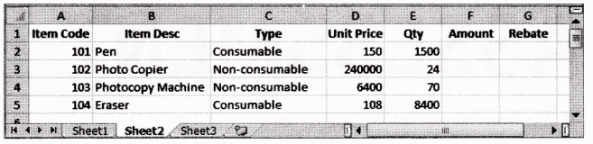
- To calculate the Amount as Unit Price*Qty for each item in Column F.
- To calculate the Rebate as 7% of Amount if Type is consumable, else calculate Rebate as 11% of Amount in Column G.
- To calculate total Rebate across all items in cell G6.
Ans :- At cell F2, type =D2*E2 and then copy this formula using mouse Fill handle onto range F3 : F5.
- At cell G2, type =IF(C2=”Consumable”, F2*0.07, F2*0.11) and then copy this formula using mouse Fill handle onto range G3 : G5.
- At cell G6, type =SUM(G2 : G5).
- To calculate the Amount as Unit Price*Qty for each item in Column F.
- Qstn #4Arihant stationery keeps stock of various stationeries in his shop. The proprietor wants to maintain a stock value and reorder level for following items as given in a spreadsheet. Write formulas for the operations (i) to (iii) and answer the questions (iv) and (v) based on the spreadsheet given below alongwith the relevant cell address:
- To calculate the Stock Value as product of ‘Quantity in Stock1 and ‘Rate’ for each item present in the spreadsheet.
- To calculate the ‘Quantity to Order’ as ‘Minimum Stock Quantity’-‘Quantity in Stock’ for each item.
- To calculate the ‘Order Value’ as product of ‘Quantity to Order’ and ‘Rate’ for the items if ‘Quantity to Order’>=0, else assign the value as 0.
- Proprietor wants to graphically represent his stationery stock. Suggest him the most appropriate feature of MS-Excel.
- If Quantity in Stock’s value changes, will have to redo all the calculations for that particular column? Explain.
Ans :- At cell F2, type = D2*E2 and then copy this formula using Fill handle in range F3 : F5.
- At cell G2, type = C2 - D2 and then copy this formula using Fill handle in range G3 : G5.
- At cell H2, type = IF (G2 > = 0, G2*E2, 0) and copy this formula using Fill handle in the range H3 : H5.
- He should create chart of any type to graphically represent his data.
- No the recalculation is not again required because the formula and functions that are given changes according to the values in the cells.
- To calculate the Stock Value as product of ‘Quantity in Stock1 and ‘Rate’ for each item present in the spreadsheet.
- Qstn #5Neha Mittal wants to store data of her montly expenditure for a period of two year and also wants to perform some calculation and analysis. Which Microsoft application, will you suggest Neha should use for this purpose and why?Ans : Microsoft Excel should be used because it cannot only be used for storing data, but also be used to perform calculations and analysis of the data.
- #Section : EMultiple Choice Questions
- Qstn #1A worksheet is a ...................
(a) collection of workbooks
(b) processing software
(c) combination of rows and columns
(d) None of the abovedigAnsr: cAns : (c) A worksheet is a combination of rows and columns.